Introduction to profile class

Example useage of Profile object.

Overview

INDEXED type class for storing data from a CTD Profile (or similar down and up observations). The structure of the class is based around having discrete profile locations with independent depth dimensions and coords. The class dataset should contain two dimensions:

> id_dim      :: The profiles dimension. Each element of this dimension
             contains data (e.g. cast) for an individual location.
> z_dim   :: The dimension for depth levels. A profile object does not
             need to have shared depths, so NaNs might be used to
             pad any depth array.

Alongside these dimensions, the following minimal coordinates should also be available:

> longitude (id_dim)   :: 1D array of longitudes, one for each id_dim
> latitude  (id_dim)   :: 1D array of latitudes, one for each id_dim
> time      (id_dim)   :: 1D array of times, one for each id_dim
> depth     (id_dim, z_dim)  :: 2D array of depths, with different depth
                            levels being provided for each profile.
                            Note that these depth levels need to be
                            stored in a 2D array, so NaNs can be used
                            to pad out profiles with shallower depths.
> id_name   (id_dim)   :: [Optional] Name of id_dim/case or id_dim number.

Introduction to Profile and ProfileAnalysis

Below is a description of the available example scripts for this class as well as an overview of validation using Profile and ProfileAnalysis.

Example Scripts

Please see COAsT/example_scripts/notesbooks/runnable_notebooks/profile_validation/*.ipynb and COAsT/example_scripts/profile_validation/*.py for some notebooks and equivalent scripts which demonstrate how to use the Profile and ProfileAnalysis classes for model validation.

1. analysis_preprocess_en4.py : If you’re using EN4 data, this kind of script might be your first step for analysis.

2. analysis_extract_and_compare.py: This script shows you how to extract the nearest model profiles, compare them with EN4 observations and get errors throughout the vertical dimension and averaged in surface and bottom zones

3. analysis_extract_and_compare_single_process.py: This script does the same as number 2. However, it is modified slightly to take a command line argument which helps it figure out which dates to analyse. This means that this script can act as a template for jug type parallel processing on, e.g. JASMIN.

4. analysis_mask_means.py: This script demonstrates how to use boolean masks to obtain regional averages of profiles and errors.

5. analysis_average_into_grid_boxes.py: This script demonstrates how to average the data inside a Profile object into regular grid boxes and seasonal climatologies.

Load and preprocess profile and model data

Start by loading python packages

import coast
from os import path
import numpy as np
import matplotlib.pyplot as plt

/usr/share/miniconda/envs/coast/lib/python3.10/site-packages/pydap/lib.py:5: DeprecationWarning: pkg_resources is deprecated as an API. See https://setuptools.pypa.io/en/latest/pkg_resources.html
/usr/share/miniconda/envs/coast/lib/python3.10/site-packages/pkg_resources/__init__.py:2871: DeprecationWarning: Deprecated call to `pkg_resources.declare_namespace('pydap')`.
Implementing implicit namespace packages (as specified in PEP 420) is preferred to `pkg_resources.declare_namespace`. See https://setuptools.pypa.io/en/latest/references/keywords.html#keyword-namespace-packages
/usr/share/miniconda/envs/coast/lib/python3.10/site-packages/pkg_resources/__init__.py:2871: DeprecationWarning: Deprecated call to `pkg_resources.declare_namespace('pydap.responses')`.
Implementing implicit namespace packages (as specified in PEP 420) is preferred to `pkg_resources.declare_namespace`. See https://setuptools.pypa.io/en/latest/references/keywords.html#keyword-namespace-packages
/usr/share/miniconda/envs/coast/lib/python3.10/site-packages/pkg_resources/__init__.py:2350: DeprecationWarning: Deprecated call to `pkg_resources.declare_namespace('pydap')`.
Implementing implicit namespace packages (as specified in PEP 420) is preferred to `pkg_resources.declare_namespace`. See https://setuptools.pypa.io/en/latest/references/keywords.html#keyword-namespace-packages
/usr/share/miniconda/envs/coast/lib/python3.10/site-packages/pkg_resources/__init__.py:2871: DeprecationWarning: Deprecated call to `pkg_resources.declare_namespace('pydap.handlers')`.
Implementing implicit namespace packages (as specified in PEP 420) is preferred to `pkg_resources.declare_namespace`. See https://setuptools.pypa.io/en/latest/references/keywords.html#keyword-namespace-packages
/usr/share/miniconda/envs/coast/lib/python3.10/site-packages/pkg_resources/__init__.py:2350: DeprecationWarning: Deprecated call to `pkg_resources.declare_namespace('pydap')`.
Implementing implicit namespace packages (as specified in PEP 420) is preferred to `pkg_resources.declare_namespace`. See https://setuptools.pypa.io/en/latest/references/keywords.html#keyword-namespace-packages
/usr/share/miniconda/envs/coast/lib/python3.10/site-packages/pkg_resources/__init__.py:2871: DeprecationWarning: Deprecated call to `pkg_resources.declare_namespace('pydap.tests')`.
Implementing implicit namespace packages (as specified in PEP 420) is preferred to `pkg_resources.declare_namespace`. See https://setuptools.pypa.io/en/latest/references/keywords.html#keyword-namespace-packages
/usr/share/miniconda/envs/coast/lib/python3.10/site-packages/pkg_resources/__init__.py:2350: DeprecationWarning: Deprecated call to `pkg_resources.declare_namespace('pydap')`.
Implementing implicit namespace packages (as specified in PEP 420) is preferred to `pkg_resources.declare_namespace`. See https://setuptools.pypa.io/en/latest/references/keywords.html#keyword-namespace-packages
/usr/share/miniconda/envs/coast/lib/python3.10/site-packages/pkg_resources/__init__.py:2871: DeprecationWarning: Deprecated call to `pkg_resources.declare_namespace('sphinxcontrib')`.
Implementing implicit namespace packages (as specified in PEP 420) is preferred to `pkg_resources.declare_namespace`. See https://setuptools.pypa.io/en/latest/references/keywords.html#keyword-namespace-packages

We can create a new Profile object easily:

profile = coast.Profile()

Currently, this object is empty, and contains no dataset. There are some reading routines currently available in Profile for reading EN4 or WOD data files. These can be used to easily read data into your new profile object:

# Read WOD data into profile object
fn_prof = path.join("example_files","WOD_example_ragged_standard_level.nc")
profile.read_wod( fn_prof )

# Read EN4 data into profile object (OVERWRITES DATASET)
fn_prof = path.join("example_files", "coast_example_en4_201008.nc")
fn_cfg_prof = path.join("config","example_en4_profiles.json")
profile = coast.Profile(config=fn_cfg_prof)
profile.read_en4( fn_prof )

config/example_en4_profiles.json

Alternatively, you can pass an xarray.dataset straight to Profile:

profile = coast.Profile( dataset = your_dataset, config = config_file [opt] )

If you are using EN4 data, you can use the process_en4() routine to apply quality control flags to the data (replacing with NaNs):

processed_profile = profile.process_en4()
profile = processed_profile

/usr/share/miniconda/envs/coast/lib/python3.10/site-packages/xarray/core/utils.py:494: FutureWarning: The return type of `Dataset.dims` will be changed to return a set of dimension names in future, in order to be more consistent with `DataArray.dims`. To access a mapping from dimension names to lengths, please use `Dataset.sizes`.
/usr/share/miniconda/envs/coast/lib/python3.10/site-packages/xarray/core/utils.py:494: FutureWarning: The return type of `Dataset.dims` will be changed to return a set of dimension names in future, in order to be more consistent with `DataArray.dims`. To access a mapping from dimension names to lengths, please use `Dataset.sizes`.

We can do some simple spatial and temporal manipulations of this data:

# Cut out a geographical box
profile = profile.subset_indices_lonlat_box(lonbounds = [-15, 15],
                                            latbounds = [45, 65])

# Cut out a time window
profile = profile.time_slice( date0 = np.datetime64('2010-01-01'), date1 = np.datetime64("2010-01-20"))

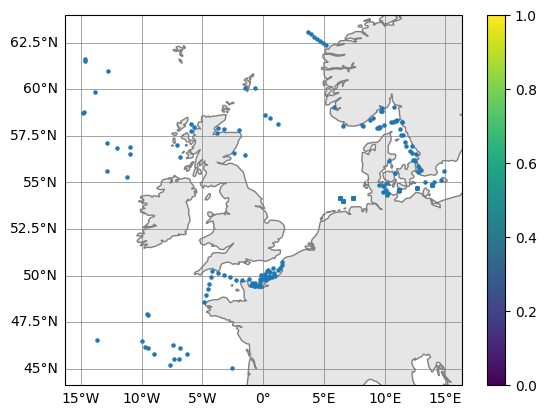
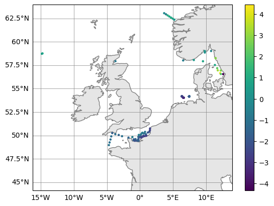
Inspect profile locations

Have a look inside the profile.py class to see what it can do

profile.plot_map()

/usr/share/miniconda/envs/coast/lib/python3.10/site-packages/cartopy/io/__init__.py:241: DownloadWarning: Downloading: https://naturalearth.s3.amazonaws.com/50m_physical/ne_50m_coastline.zip

(<Figure size 640x480 with 2 Axes>, <GeoAxes: >)

Direct Model comparison using obs_operator() method

There are a number of routines available for interpolating in the horizontal, vertical and in time to do direct comparisons of model and profile data. Profile.obs_operator will do a nearest neighbour spatial interpolation of the data in a Gridded object to profile latitudes/longitudes. It will also do a custom time interpolation.

First load some model data:

root = "./"
# And by defining some file paths
dn_files = root + "./example_files/"
fn_nemo_dat = path.join(dn_files, "coast_example_nemo_data.nc")
fn_nemo_dom = path.join(dn_files, "coast_example_nemo_domain.nc")
fn_nemo_config = path.join(root, "./config/example_nemo_grid_t.json")

# Create gridded object:
nemo = coast.Gridded(fn_nemo_dat, fn_nemo_dom, multiple=True, config=fn_nemo_config)

/usr/share/miniconda/envs/coast/lib/python3.10/site-packages/xarray/core/dataset.py:282: UserWarning: The specified chunks separate the stored chunks along dimension "time_counter" starting at index 2. This could degrade performance. Instead, consider rechunking after loading.

Create a landmask array in Gridded

In this example we add a landmask variable to the Gridded dataset. When this is present, the obs_operator will use this to interpolation to the nearest wet point. If not present, it will just take the nearest grid point (not implemented).

We also rename the depth at initial time coordinate depth_0 to depth as this is expected by Profile()

nemo.dataset["landmask"] = nemo.dataset.bottom_level == 0
nemo.dataset = nemo.dataset.rename({"depth_0": "depth"})  # profile methods will expect a `depth` coordinate

Interpolate model to horizontal observation locations using obs_operator() method

# Use obs operator for horizontal remapping of Gridded onto Profile.
model_profiles = profile.obs_operator(nemo)

/usr/share/miniconda/envs/coast/lib/python3.10/site-packages/xarray/core/utils.py:494: FutureWarning: The return type of `Dataset.dims` will be changed to return a set of dimension names in future, in order to be more consistent with `DataArray.dims`. To access a mapping from dimension names to lengths, please use `Dataset.sizes`.
/usr/share/miniconda/envs/coast/lib/python3.10/site-packages/xarray/core/utils.py:494: FutureWarning: The return type of `Dataset.dims` will be changed to return a set of dimension names in future, in order to be more consistent with `DataArray.dims`. To access a mapping from dimension names to lengths, please use `Dataset.sizes`.
/usr/share/miniconda/envs/coast/lib/python3.10/site-packages/coast/data/profile.py:456: UserWarning: Converting non-nanosecond precision timedelta values to nanosecond precision. This behavior can eventually be relaxed in xarray, as it is an artifact from pandas which is now beginning to support non-nanosecond precision values. This warning is caused by passing non-nanosecond np.datetime64 or np.timedelta64 values to the DataArray or Variable constructor; it can be silenced by converting the values to nanosecond precision ahead of time.
/usr/share/miniconda/envs/coast/lib/python3.10/site-packages/coast/data/profile.py:456: UserWarning: Converting non-nanosecond precision timedelta values to nanosecond precision. This behavior can eventually be relaxed in xarray, as it is an artifact from pandas which is now beginning to support non-nanosecond precision values. This warning is caused by passing non-nanosecond np.datetime64 or np.timedelta64 values to the DataArray or Variable constructor; it can be silenced by converting the values to nanosecond precision ahead of time.

Now that we have interpolated the model onto Profiles, we have a new Profile object called model_profiles. This can be used to do some comparisons with our original processed_profile object, which we created above.

Discard profiles where the interpolation distance is too large

However maybe we first want to restrict the set of model profiles to those that were close to the observations; perhaps, for example, the observational profiles are beyond the model domain. The model resolution would be an appropriate scale to pick

too_far = 7  # distance km
keep_indices = model_profiles.dataset.interp_dist <= too_far
model_profiles = model_profiles.isel(id_dim=keep_indices)

# Also drop the unwanted observational profiles
profile = profile.isel(id_dim=keep_indices)

Profile analysis

Create an object for Profile analysis

Let’s make our ProfileAnalysis object:

analysis = coast.ProfileAnalysis()

We can use ProfileAnalysis.interpolate_vertical to interpolate all variables within a Profile object. This can be done onto a set of reference depths or, matching another object’s depth coordinates by passing another profile object. Let’s interpolate our model profiles onto observations depths, then interpolate both onto a set of reference depths:

### Set depth averaging settings
ref_depth = np.concatenate((np.arange(1, 100, 2), np.arange(100, 300, 5), np.arange(300, 1000, 50)))

# Interpolate model profiles onto observation depths
model_profiles_interp = analysis.interpolate_vertical(model_profiles, profile, interp_method="linear")

# Vertical interpolation of model profiles to reference depths
model_profiles_interp_ref = analysis.interpolate_vertical(model_profiles_interp, ref_depth)

# Interpolation of obs profiles to reference depths
profile_interp_ref = analysis.interpolate_vertical(profile, ref_depth)

However, there is a problem here as the interpolate_vertical() method tries to map the whole contents of profile to the ref_depth and the profile object contains some binary data from the original qc flags. The data from the qc flags was mapped using process_en4() so the original qc entries can be removed.

## Strip out old QC variables
profile.dataset = profile.dataset.drop_vars(['qc_potential_temperature','qc_practical_salinity',
                                 'qc_depth','qc_time',
                                 'qc_flags_profiles','qc_flags_levels'])

# Interpolation of obs profiles to reference depths
profile_interp_ref = analysis.interpolate_vertical(profile, ref_depth)

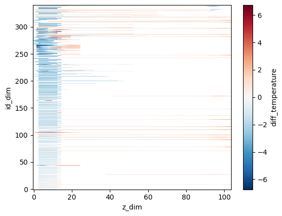
Differencing

Now that we have two Profile objects that are horizontally and vertically comparable, we can use difference() to get some basic errors:

differences = analysis.difference(profile_interp_ref, model_profiles_interp_ref)

This will return a new Profile object that contains the variable difference, absolute differences and square differences at all depths and means for each profile.

Type

differences.dataset

to see what it returns

# E.g. plot the differences on ind_dim vs z_dim axes
differences.dataset.diff_temperature.plot()

<matplotlib.collections.QuadMesh at 0x7f50f5e56e00>

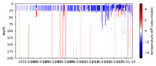
# or a bit prettier on labelled axes
cmap=plt.get_cmap('seismic')
fig = plt.figure(figsize=(8, 3))

plt.pcolormesh( differences.dataset.time, ref_depth, differences.dataset.diff_temperature.T,
                    label='abs_diff', cmap=cmap,
                    vmin=-5, vmax=5)
plt.ylim([0,200])
plt.gca().invert_yaxis()
plt.ylabel('depth')
plt.colorbar( label='temperature diff (obs-model)')

<matplotlib.colorbar.Colorbar at 0x7f50f4c0c370>

Layer Averaging

We can use the Profile object to get mean values between specific depth levels or for some layer above the bathymetric depth. The former can be done using ProfileAnalysis.depth_means(), for example the following will return a new Profile object containing the means of all variables between 0m and 5m:

profile_surface = analysis.depth_means(profile, [0, 5])  # 0 - 5 metres

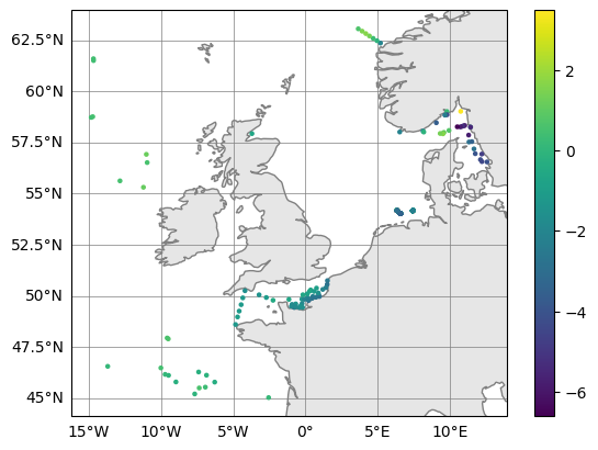
But since this can work on any Profile object it would be more interesting to apply it to the differences between the interpolated observations and model points

surface_def = 10  # in metres

model_profiles_surface = analysis.depth_means(model_profiles_interp_ref, [0, surface_def])
obs_profiles_surface   = analysis.depth_means(profile_interp_ref, [0, surface_def])
surface_errors = analysis.difference(obs_profiles_surface, model_profiles_surface)

# Plot (observation - model) upper 10m averaged temperatures
surface_errors.plot_map(var_str="diff_temperature")

(<Figure size 640x480 with 2 Axes>, <GeoAxes: >)

This can be done for any arbitrary depth layer defined by two depths.

However, in some cases it may be that one of the depth levels is not defined by a constant, e.g. when calculating bottom means. In this case you may want to calculate averages over a height from the bottom that is conditional on the bottom depth. This can be done using ProfileAnalysis.bottom_means(). For example:

bottom_height = [10, 50, 100]  # Average over bottom heights of 10m, 30m and 100m for...
bottom_thresh = [100, 500, np.inf]  # ...bathymetry depths less than 100m, 100-500m and 500-infinite
model_profiles_bottom = analysis.bottom_means(model_profiles_interp_ref, bottom_height, bottom_thresh)

similarly compute the same for the observations… though first we have to patch in a bathymetry variable that will be expected by the method. Grab it from the model dataset.

profile_interp_ref.dataset["bathymetry"] = (["id_dim"], model_profiles_interp_ref.dataset["bathymetry"].values)
obs_profiles_bottom = analysis.bottom_means(profile_interp_ref, bottom_height, bottom_thresh)

Now the difference can be calculated

bottom_errors = analysis.difference( obs_profiles_bottom, model_profiles_bottom)

# Plot (observation - model) upper 10m averaged temperatures
bottom_errors.plot_map(var_str="diff_temperature")

(<Figure size 640x480 with 2 Axes>, <GeoAxes: >)

NOTE1: The bathymetry variable does not actually need to contain bathymetric depths, it can also be used to calculate means above any non-constant surface. For example, it could be mixed layer depth.

NOTE2: This can be done for any Profile object. So, you could use this workflow to also average a Profile derived from the difference() routine.

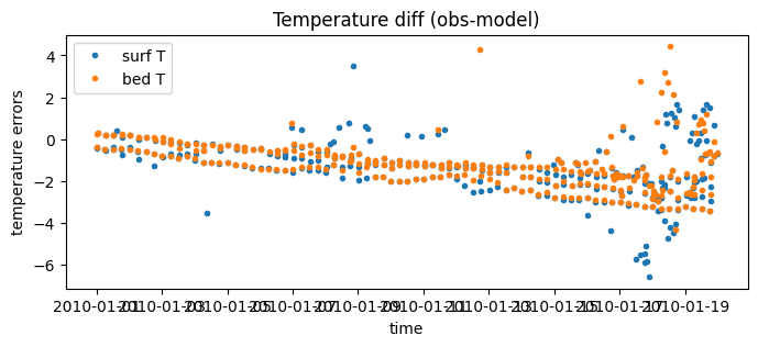
# Since they are indexed by 'id_dim' they can be plotted against time
fig = plt.figure(figsize=(8, 3))

plt.plot( surface_errors.dataset.time, surface_errors.dataset.diff_temperature, '.', label='surf T' )
plt.plot( bottom_errors.dataset.time, bottom_errors.dataset.diff_temperature, '.', label='bed T' )
plt.xlabel('time')
plt.ylabel('temperature errors')
plt.legend()
plt.title("Temperature diff (obs-model)")

Text(0.5, 1.0, 'Temperature diff (obs-model)')

Regional (Mask) Averaging

We can use Profile in combination with MaskMaker to calculate averages over regions defined by masks. For example, to get the mean errors in the North Sea. Start by creating a list of boolean masks we would like to use:

mm = coast.MaskMaker()

# Define Regional Masks
regional_masks = []

# Define convenient aliases based on nemo data
lon = nemo.dataset.longitude.values
lat = nemo.dataset.latitude.values
bathy = nemo.dataset.bathymetry.values

# Add regional mask for whole domain
regional_masks.append(np.ones(lon.shape))

# Add regional mask for English Channel
regional_masks.append(mm.region_def_nws_english_channel(lon, lat, bathy))
region_names = ["whole_domain","english_channel",]

Next, we must make these masks into datasets using MaskMaker.make_mask_dataset. Masks should be 2D datasets defined by booleans. In our example here we have used the latitude/longitude array from the nemo object, however it can be defined however you like.

mask_list = mm.make_mask_dataset(lon, lat, regional_masks)

Then we use ProfileAnalysis.determine_mask_indices to figure out which profiles in a Profile object lie within each regional mask:

mask_indices = analysis.determine_mask_indices(profile, mask_list)

This returns an object called mask_indices, which is required to pass to ProfileAnalysis.mask_means(). This routine will return a new xarray dataset containing averaged data for each region:

mask_means = analysis.mask_means(profile, mask_indices)

/usr/share/miniconda/envs/coast/lib/python3.10/site-packages/xarray/core/utils.py:494: FutureWarning: The return type of `Dataset.dims` will be changed to return a set of dimension names in future, in order to be more consistent with `DataArray.dims`. To access a mapping from dimension names to lengths, please use `Dataset.sizes`.

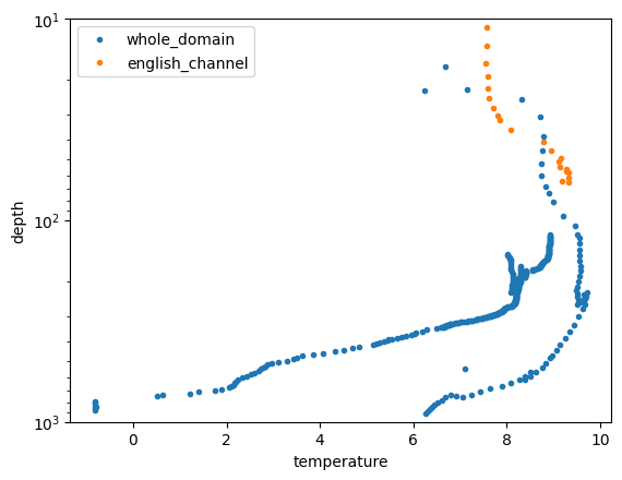
which can be visualised or further processed

for count_region in range(len(region_names)):
    plt.plot( mask_means.profile_mean_temperature.isel(dim_mask=count_region),
          mask_means.profile_mean_depth.isel(dim_mask=count_region),
          label=region_names[count_region],
          marker=".", linestyle='none')

plt.ylim([10,1000])
plt.yscale("log")
plt.gca().invert_yaxis()
plt.xlabel('temperature'); plt.ylabel('depth')
plt.legend()

<matplotlib.legend.Legend at 0x7f50f4af8250>

Gridding Profile Data

If you have large amount of profile data you may want to average it into grid boxes to get, for example, mean error maps or climatologies. This can be done using ProfileAnalysis.average_into_grid_boxes().

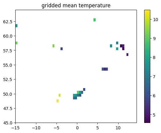
We can create a gridded dataset shape (y_dim, x_dim) from all the data using:

grid_lon = np.arange(-15, 15, 0.5)
grid_lat = np.arange(45, 65, 0.5)
prof_gridded = analysis.average_into_grid_boxes(profile, grid_lon, grid_lat)
# NB this method does not separately treat `z_dim`, see docstr

lat = prof_gridded.dataset.latitude
lon = prof_gridded.dataset.longitude
temperature = prof_gridded.dataset.temperature

plt.pcolormesh( lon, lat, temperature)
plt.title('gridded mean temperature')
plt.colorbar()

<matplotlib.colorbar.Colorbar at 0x7f50f46e6e30>

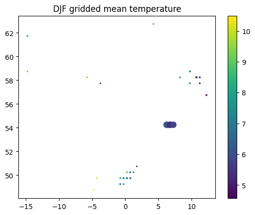
Alternatively, we can calculate averages for each season:

prof_gridded_DJF = analysis.average_into_grid_boxes(profile, grid_lon, grid_lat, season="DJF", var_modifier="_DJF")
prof_gridded_MAM = analysis.average_into_grid_boxes(profile, grid_lon, grid_lat, season="MAM", var_modifier="_MAM")
prof_gridded_JJA = analysis.average_into_grid_boxes(profile, grid_lon, grid_lat, season="JJA", var_modifier="_JJA")
prof_gridded_SON = analysis.average_into_grid_boxes(profile, grid_lon, grid_lat, season="SON", var_modifier="_SON")

Here, season specifies which season to average over and var_modifier is added to the end of all variable names in the object’s dataset.

NB with the example data only DJF has any data.

This function returns a new Gridded object. It also contains a new variable called grid_N, which stores how many profiles were averaged into each grid box. You may want to use this when using or extending the analysis. E.g. use it with plot symbol size

temperature = prof_gridded_DJF.dataset.temperature_DJF
N = prof_gridded_DJF.dataset.grid_N_DJF
plt.scatter( lon, lat, c=temperature, s=N)
plt.title('DJF gridded mean temperature')
plt.colorbar()

<matplotlib.colorbar.Colorbar at 0x7f50f45ee170>