Zarr files

Zarr files example.

8 minute read

Load Zarr files

This tutorial will show some examples on how to load zarr files on coast. It will include:

Creation of a Gridded object
Loading data into the Gridded object.
Combining Gridded output and Gridded domain data.
Interrogating the Gridded object.
Basic manipulation and subsetting
Looking at the data with matplotlib

Requirements

Coast also has the capability to allow you to open zarr files In order to do that, you need to install first the library zarr:

pip install zarr xarray[complete] aiohttp requests

After that, you can open the datasets

Import

Begin by importing COAsT and define some file paths for NEMO output data and a NEMO domain, as an example of model data suitable for the Gridded object.

import coast
import matplotlib.pyplot as plt
import datetime
import numpy as np
import xarray as xr
import zarr

root = "./"
fn_config_t_grid = root + "./config/example_nemo_monthly_climate.json"

# Define some file paths
fn_nemo_dom_mask = "https://noc-msm-o.s3-ext.jc.rl.ac.uk/n06-coast-testing/mask.zarr"
fn_nemo_dom_mesh_zgr = "https://noc-msm-o.s3-ext.jc.rl.ac.uk/n06-coast-testing/mesh_zgr.zarr"
fn_nemo_dom_mesh_hgr = "https://noc-msm-o.s3-ext.jc.rl.ac.uk/n06-coast-testing/mesh_hgr.zarr"
fn_nemo_dat_t = "https://noc-msm-o.s3-ext.jc.rl.ac.uk/n06-coast-testing/n06_T.zarr"
fn_nemo_dat_u = "https://noc-msm-o.s3-ext.jc.rl.ac.uk/n06-coast-testing/n06_U.zarr"
fn_nemo_dat_v = "https://noc-msm-o.s3-ext.jc.rl.ac.uk/n06-coast-testing/n06_V.zarr"

/mnt/code/.pyenv/versions/3.10.12/envs/coast-10/lib/python3.10/site-packages/utide/harmonics.py:16: RuntimeWarning: invalid value encountered in cast
/mnt/code/.pyenv/versions/3.10.12/envs/coast-10/lib/python3.10/site-packages/utide/harmonics.py:17: RuntimeWarning: invalid value encountered in cast

Open the zarr files as a XARRAY

The zarr files that we are using in this example do not have all the variables on the same file. Because of that, we need to open each file separately and then add the variables to a central file

dom = xr.open_zarr(fn_nemo_dom_mask)
mesh_zgr = xr.open_zarr(fn_nemo_dom_mesh_zgr)
mesh_hgr = xr.open_zarr(fn_nemo_dom_mesh_hgr)

/tmp/ipykernel_262236/396929176.py:1: RuntimeWarning: Failed to open Zarr store with consolidated metadata, but successfully read with non-consolidated metadata. This is typically much slower for opening a dataset. To silence this warning, consider:
1. Consolidating metadata in this existing store with zarr.consolidate_metadata().
2. Explicitly setting consolidated=False, to avoid trying to read consolidate metadata, or
3. Explicitly setting consolidated=True, to raise an error in this case instead of falling back to try reading non-consolidated metadata.

for var_name in mesh_zgr.data_vars:
    dom[var_name] = mesh_zgr[var_name]
for var_name in mesh_hgr.data_vars:
    dom[var_name] = mesh_hgr[var_name]

u_grid = xr.open_zarr(fn_nemo_dat_u)
u_grid = u_grid.isel(time_counter=slice(0,119)).rename({'depthu': 'depth'})
v_grid = xr.open_zarr(fn_nemo_dat_v)
v_grid = v_grid.isel(time_counter=slice(0,119)).rename({'depthv': 'depth'})
t_grid = xr.open_zarr(fn_nemo_dat_t)
t_grid = t_grid.rename({'deptht': 'depth'})

for var_name in u_grid.data_vars:
    t_grid[var_name] = u_grid[var_name]
for var_name in v_grid.data_vars:
    t_grid[var_name] = v_grid[var_name]

/mnt/code/.pyenv/versions/3.10.12/envs/coast-10/lib/python3.10/site-packages/dask/array/core.py:4836: PerformanceWarning: Increasing number of chunks by factor of 15
/mnt/code/.pyenv/versions/3.10.12/envs/coast-10/lib/python3.10/site-packages/dask/array/core.py:4836: PerformanceWarning: Increasing number of chunks by factor of 15

#Uncomment to see the data
# dom

#Uncomment to see the data
# t_grid

Slice the zarr files

Because zarr files are optimized for cloud, when we instantiate an xarray dataset, we do not open the zarr by it self. We only open some metadata related to the file. The files will only be downloaed when we need to perform some processing on the data

dom = dom.isel(y=slice(500, 700), x=slice(1000,1200))

t_grid = t_grid.isel(y=slice(500, 700), x=slice(1000,1200), time_counter=slice(0,24))

Loading and Interrogating

We can create a new Gridded object by simple calling coast.Gridded(). By passing this a NEMO data file and a NEMO domain file, COAsT will combine the two into a single xarray dataset within the Gridded object. Each individual Gridded object should be for a specified NEMO grid type, which is specified in a configuration file which is also passed as an argument. The Dask library is switched on by default, chunking can be specified in the configuration file.

nemo_t = coast.Gridded(fn_data= t_grid, fn_domain = dom, config=fn_config_t_grid)

/mnt/code/code/noc/coast/COAsT/coast/data/gridded.py:236: UserWarning: The model domain loaded, '<xarray.Dataset>
Dimensions:       (t: 1, z: 75, y: 200, x: 200)
Dimensions without coordinates: t, z, y, x
Data variables: (12/34)
    e3t_0         (t, z, y, x) float64 dask.array<chunksize=(1, 5, 76, 82), meta=np.ndarray>
    e3t_1d        (t, z) float64 dask.array<chunksize=(1, 75), meta=np.ndarray>
    e3u_0         (t, z, y, x) float64 dask.array<chunksize=(1, 5, 76, 82), meta=np.ndarray>
    e3v_0         (t, z, y, x) float64 dask.array<chunksize=(1, 5, 76, 82), meta=np.ndarray>
    e3w_0         (t, z, y, x) float64 dask.array<chunksize=(1, 5, 76, 82), meta=np.ndarray>
    e3w_1d        (t, z) float64 dask.array<chunksize=(1, 75), meta=np.ndarray>
    ...            ...
    glamu         (t, y, x) float32 dask.array<chunksize=(1, 200, 82), meta=np.ndarray>
    glamv         (t, y, x) float32 dask.array<chunksize=(1, 200, 82), meta=np.ndarray>
    gphif         (t, y, x) float32 dask.array<chunksize=(1, 200, 82), meta=np.ndarray>
    gphit         (t, y, x) float32 dask.array<chunksize=(1, 200, 82), meta=np.ndarray>
    gphiu         (t, y, x) float32 dask.array<chunksize=(1, 200, 82), meta=np.ndarray>
    gphiv         (t, y, x) float32 dask.array<chunksize=(1, 200, 82), meta=np.ndarray>
Attributes:
    DOMAIN_number_total:  8972
    DOMAIN_size_global:   [4322, 3059]', does not contain the bathy_metry' variable. This will result in the NEMO.dataset.bathymetry variable being set to zero, which may result in unexpected behaviour from routines that require this variable.

!IMPORTANT!: this dataset does not contain bathymetry data.

Our new Gridded object nemo_t contains a variable called dataset, which holds information on the two files we passed. Let’s have a look at this:

# nemo_t.dataset # uncomment to print data object summary

This is an xarray dataset, which has all the information on netCDF style structures. You can see dimensions, coordinates and data variables. At the moment, none of the actual data is loaded to memory and will remain that way until it needs to be accessed.

As it is a zarr file, it will only get any data if you apply compute() on the data:

ssh = nemo_t.dataset.ssh
ssh.compute()
# ssh # uncomment to print data object summary

<xarray.DataArray 'ssh' (t_dim: 24, y_dim: 200, x_dim: 200)>
array([[[-1.6210064 , -1.6217471 , -1.6231693 , …, -1.5842544 ,
-1.5886359 , -1.5930159 ],
[-1.6208621 , -1.6217225 , -1.6233234 , …, -1.5888053 ,
-1.5935609 , -1.5981766 ],
[-1.621304  , -1.6223003 , -1.6240481 , …, -1.5930148 ,
-1.5981003 , -1.6029042 ],
…,
[-0.98735386, -0.9597808 , -0.931632  , …, -0.6270069 ,
-0.6278365 , -0.6290987 ],
[-1.0102477 , -0.9808094 , -0.9505175 , …, -0.63027424,
-0.6316009 , -0.63331974],
[-1.0307174 , -0.99985355, -0.96790063, …, -0.63465285,
-0.6367161 , -0.6389442 ]],
   [[-1.6141921 , -1.6149583 , -1.6157647 , ..., -1.5382599 ,
     -1.5428585 , -1.5479578 ],
    [-1.6137543 , -1.614481  , -1.6153185 , ..., -1.5421394 ,
     -1.5469443 , -1.5521828 ],
    [-1.6131831 , -1.6138711 , -1.6147525 , ..., -1.5456467 ,
     -1.5506693 , -1.5560651 ],
…
[-0.5291973 , -0.53182423, -0.537423 , …, -0.7970734 ,
-0.8119881 , -0.82499063],
[-0.53454167, -0.5373199 , -0.54308665, …, -0.77014893,
-0.7829233 , -0.7941438 ],
[-0.53937477, -0.5424393 , -0.5484757 , …, -0.7462123 ,
-0.7570849 , -0.76668566]],
   [[-1.6791433 , -1.6803815 , -1.6808515 , ..., -1.5127497 ,
     -1.5175854 , -1.5226325 ],
    [-1.679447  , -1.6804127 , -1.6806444 , ..., -1.5093309 ,
     -1.5140619 , -1.5190879 ],
    [-1.6797307 , -1.6804144 , -1.6804197 , ..., -1.5054852 ,
     -1.5097626 , -1.5145139 ],
    ...,
    [-0.67837346, -0.6714207 , -0.6632468 , ..., -0.77248365,
     -0.79867   , -0.82295316],
    [-0.6826826 , -0.6778399 , -0.67128325, ..., -0.74587363,
     -0.7708025 , -0.794183  ],
    [-0.68843955, -0.68585885, -0.681205  , ..., -0.71919113,
     -0.7428356 , -0.7651531 ]]], dtype=float32)
Coordinates:
time (t_dim) datetime64[ns] 1960-01-06T12:00:00 … 1961-12-13T22:1…
longitude (y_dim, x_dim) float32 156.2 156.3 156.4 … 172.7 172.8 172.8
latitude (y_dim, x_dim) float32 -63.49 -63.49 -63.49 … -55.07 -55.07
Dimensions without coordinates: t_dim, y_dim, x_dim
Attributes:
interval_operation: 300s
interval_write: 1mo
long_name: sea_surface_height_above_geoid
online_operation: average
units: m

Or as a numpy array:

ssh_np = ssh.values
#ssh_np.shape # uncomment to print data object summary

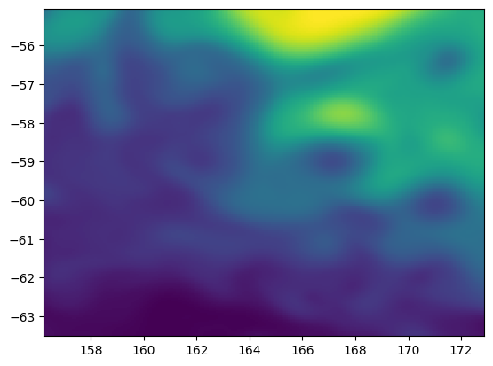
Then lets plot up a single time snapshot of ssh using matplotlib:

plt.pcolormesh(nemo_t.dataset.longitude, nemo_t.dataset.latitude, nemo_t.dataset.ssh[0])

<matplotlib.collections.QuadMesh at 0x7fa6e3d77a60>

png

Feedback

Was this page helpful?

Glad to hear it!

Sorry to hear that. Please tell us how we can improve.

Last modified December 11, 2023: add configuration gallery (0696a01)