Example scripts and Gallery
Example scripts and gallery for other NEMO configurations. Scripts from example_scripts
5 minute read
Polar plotting example
"""
polar_plotting.py
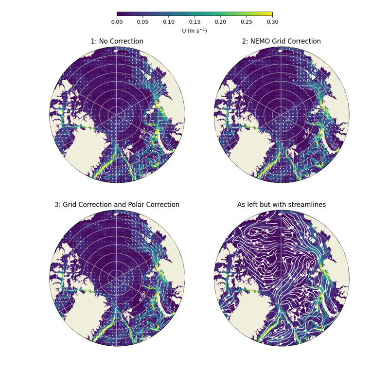
This demonstration will show how to re-project the NEMO velocities for quiver
plotting in polar coordinates.
"""
#%%
import coast
import numpy as np
import xarray as xr
import matplotlib.pyplot as plt
import matplotlib.colors as colors # colormap fiddling
#################################################
#%% Loading data
#################################################
import matplotlib.pyplot as plt
import cartopy.crs as ccrs
import cartopy.feature as cfeature
import coast
#################################################
# Usage of coast._utils.plot_util.velocity_grid_to_geo()
# Plotting velocities with curvilinear grid and/or on a polar stereographic projection.
#################################################
root = "./"
# Paths to a single or multiple data files.
dn_files = root + "example_files/"
fn_nemo_dat_t = dn_files + "coast_nemo_quiver_thetao.nc"
fn_nemo_dat_u = dn_files + "coast_nemo_quiver_uo.nc"
fn_nemo_dat_v = dn_files + "coast_nemo_quiver_vo.nc"
fn_nemo_config_t = root + "config/gc31_nemo_grid_t.json"
fn_nemo_config_u = root + "config/gc31_nemo_grid_u.json"
fn_nemo_config_v = root + "config/gc31_nemo_grid_v.json"
# Set path for domain file if required.
fn_nemo_dom = dn_files + "coast_nemo_quiver_dom.nc"
# Define output filepath (optional: None or str)
fn_out = './quiver_plot.png'
# Read in multiyear data (This example uses NEMO data from a single file.)
nemo_data_t = coast.Gridded(fn_data=fn_nemo_dat_t,
fn_domain=fn_nemo_dom,
config=fn_nemo_config_t,
).dataset
nemo_data_u = coast.Gridded(fn_data=fn_nemo_dat_u,
fn_domain=fn_nemo_dom,
config=fn_nemo_config_u,
).dataset
nemo_data_v = coast.Gridded(fn_data=fn_nemo_dat_v,
fn_domain=fn_nemo_dom,
config=fn_nemo_config_v,
).dataset
# Select surface u and v as an example:
data_u = nemo_data_u[["u_velocity"]]
data_v = nemo_data_v[["v_velocity"]]
# Select one time step and surface currents
data_u = data_u.isel(t_dim=0, z_dim=0)
data_v = data_v.isel(t_dim=0, z_dim=0)
# Calculate speed
speed = ((data_u.to_array().values[0, :, :] ** 2 + data_v.to_array().values[0, :, :] ** 2) ** 0.5)
# Calculate adjustment for the curvilinear grid
# This function may take a while
uv_velocities = [data_u.to_array().values[0, :, :], data_v.to_array().values[0, :, :]]
u_new, v_new = coast._utils.plot_util.velocity_grid_to_geo(
nemo_data_t.longitude.values, nemo_data_t.latitude.values,
uv_velocities,
polar_stereo_cartopy_bug_fix=False)
# Apply the CartoPy stereographic polar correction
# NOTE: This could have been applied automatically with `polar_stereo=True` in
# coast._utils.plot_util.velocity_grid_to_geo()
u_pol, v_pol = coast._utils.plot_util.velocity_polar_bug_fix(u_new, v_new, nemo_data_t.latitude.values)
# Set things up for plotting North Pole stereographic projection
# Data projection
data_crs = ccrs.PlateCarree()
# Plot projection
mrc = ccrs.NorthPolarStereo(central_longitude=0.0)
#################################################
# Below shows the u and v velocities when plotted with and without adjustment.
# The plot shows three cases: 1:no correction, 2:the NEMO grid correction, and 3:
# the NEMO grid correction with polar stereographic plot correction. We also plot
# the final corrected u and v velocities as streamlines.
#
# In case 1, the lower latitude velocities aren't too bad but become irregular
# further north as the grid lines deviate form lat and lon.
#
# In case 2, the irregularity still persists even with the grid correction. This
# is the result of a CartoPy bug which also worsens at high latitudes.
#
# In case 3, both corrections have been applied and the velocities quivers now align
# with the route of strong current speed as would be expected.
#################################################
# Subplot axes settings
n_r = 2 # Number of subplot rows
n_c = 2 # Number of subplot columns
figsize = (20, 20) # Figure size
subplot_padding = 0.5 # Amount of vertical and horizontal padding between plots
fig_pad = (0.075, 0.075, 0.1, 0.1) # Figure padding (left, top, right, bottom)
# Labels and Titles
fig_title = "Velocity Plot" # Whole figure title
# Create plot and flatten axis array
fig, ax = plt.subplots(n_r, n_c, subplot_kw={"projection": mrc}, sharey=True, sharex=True, figsize=figsize)
cax = fig.add_axes([0.3, 0.96, 0.4, 0.01])
ax = ax.flatten()
for rr in range(n_r * n_c):
ax[rr].add_feature(cfeature.LAND, zorder=100)
ax[rr].gridlines()
ax[rr].set_extent([-180, 180, 70, 90], crs=data_crs)
coast._utils.plot_util.set_circle(ax[rr])
cs = ax[0].pcolormesh(nemo_data_t.longitude.values, nemo_data_t.latitude.values, speed, transform=data_crs, vmin=0, vmax=0.3)
ax[0].quiver(nemo_data_t.longitude.values, nemo_data_t.latitude.values,
data_u.to_array().values[0, :, :], data_v.to_array().values[0, :, :],
color='w', transform=data_crs, angles='xy', regrid_shape=40)
ax[1].pcolormesh(nemo_data_t.longitude.values, nemo_data_t.latitude.values, speed, transform=data_crs, vmin=0, vmax=0.3)
ax[1].quiver(nemo_data_t.longitude.values, nemo_data_t.latitude.values,
u_new, v_new,
color='w', transform=data_crs, angles='xy', regrid_shape=40)
ax[2].pcolormesh(nemo_data_t.longitude.values, nemo_data_t.latitude.values, speed, transform=data_crs, vmin=0, vmax=0.3)
ax[2].quiver(nemo_data_t.longitude.values, nemo_data_t.latitude.values,
u_pol, v_pol,
color='w', transform=data_crs, angles='xy', regrid_shape=40)
ax[3].pcolormesh(nemo_data_t.longitude.values, nemo_data_t.latitude.values, speed, transform=data_crs, vmin=0, vmax=0.3)
ax[3].streamplot(nemo_data_t.longitude.values, nemo_data_t.latitude.values,
u_pol, v_pol, transform=data_crs, linewidth=1, density=2, color='w', zorder=101)
ax[0].set_title('1: No Correction')
ax[1].set_title('2: NEMO Grid Correction')
ax[2].set_title('3: Grid Correction and Polar Correction')
ax[3].set_title('As left but with streamlines')
fig.colorbar(cs, cax=cax, orientation='horizontal')
cax.set_xlabel('U (m s$^{-1}$)')
#fig.tight_layout(w_pad=subplot_padding, h_pad=subplot_padding)
#fig.subplots_adjust(left=(fig_pad[0]), bottom=(fig_pad[1]), right=(1 - fig_pad[2]), top=(1 - fig_pad[3]))
plt.show()
# uncomment this line to save an output image
fig.savefig(fn_out)
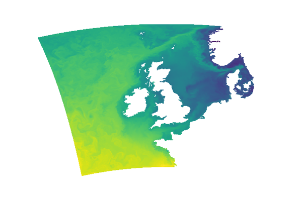
AMM15 - 1.5km resolution Atlantic Margin Model
"""
AMM15_example_plot.py

Make simple AMM15 SST plot.

"""

#%%
import coast
import numpy as np
import xarray as xr
import matplotlib.pyplot as plt
import matplotlib.colors as colors # colormap fiddling

#################################################
#%%  Loading  data
#################################################


config = 'AMM15'
dir_nam = "/projectsa/NEMO/gmaya/2013p2/"
fil_nam = "20130415_25hourm_grid_T.nc"
dom_nam = "/projectsa/NEMO/gmaya/AMM15_GRID/amm15.mesh_mask.cs3x.nc"
config = "/work/jelt/GitHub/COAsT/config/example_nemo_grid_t.json"

sci_t = coast.Gridded(dir_nam + fil_nam, dom_nam, config=config)  # , chunks=chunks)
chunks = {
    "x_dim": 10,
    "y_dim": 10,
    "t_dim": 10,
}  # Chunks are prescribed in the config json file, but can be adjusted while the data is lazy loaded.

sci_t.dataset.chunk(chunks)

# create an empty w-grid object, to store stratification
sci_w = coast.Gridded(fn_domain=dom_nam, config=config.replace("t_nemo", "w_nemo"))
sci_w.dataset.chunk({"x_dim": 10, "y_dim": 10})  # Can reset after loading config json

print('* Loaded ',config, ' data')

#################################################
#%% subset of data and domain ##
#################################################
# Pick out a North Sea subdomain
print('* Extract North Sea subdomain')
ind_sci = sci_t.subset_indices([51,-4], [62,15])
sci_nwes_t = sci_t.isel(y_dim=ind_sci[0], x_dim=ind_sci[1]) #nwes = northwest europe shelf
ind_sci = sci_w.subset_indices([51,-4], [62,15])
sci_nwes_w = sci_w.isel(y_dim=ind_sci[0], x_dim=ind_sci[1]) #nwes = northwest europe shelf

#%% Apply masks to temperature and salinity
if config == 'AMM15':
    sci_nwes_t.dataset['temperature_m'] = sci_nwes_t.dataset.temperature.where( sci_nwes_t.dataset.mask.expand_dims(dim=sci_nwes_t.dataset['t_dim'].sizes) > 0)
    sci_nwes_t.dataset['salinity_m'] = sci_nwes_t.dataset.salinity.where( sci_nwes_t.dataset.mask.expand_dims(dim=sci_nwes_t.dataset['t_dim'].sizes) > 0)

else:
    # Apply fake masks to temperature and salinity
    sci_nwes_t.dataset['temperature_m'] = sci_nwes_t.dataset.temperature
    sci_nwes_t.dataset['salinity_m'] = sci_nwes_t.dataset.salinity


#%% Plots
fig = plt.figure()

plt.pcolormesh( sci_t.dataset.longitude, sci_t.dataset.latitude, sci_t.dataset.temperature.isel(z_dim=0).squeeze())
#plt.xlabel('longitude')
#plt.ylabel('latitude')
#plt.colorbar()
plt.axis('off')
plt.show()


fig.savefig('AMM15_SST_nocolorbar.png', dpi=120)
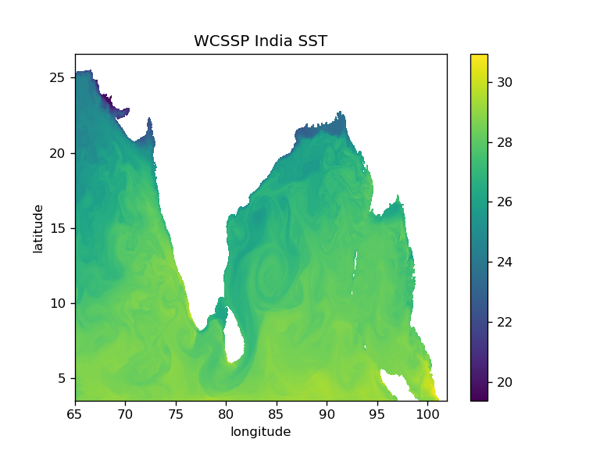
India subcontinent maritime domain. WCSSP India configuration
#%%
import coast
import numpy as np
import xarray as xr
import dask
import matplotlib.pyplot as plt
import matplotlib.colors as colors # colormap fiddling

#################################################
#%%  Loading  data
#################################################


dir_nam = "/projectsa/COAsT/NEMO_example_data/MO_INDIA/"
fil_nam = "ind_1d_cat_20180101_20180105_25hourm_grid_T.nc"
dom_nam = "domain_cfg_wcssp.nc"
config_t = "/work/jelt/GitHub/COAsT/config/example_nemo_grid_t.json"

sci_t = coast.Gridded(dir_nam + fil_nam, dir_nam + dom_nam, config=config_t)

#%% Plot
fig = plt.figure()

plt.pcolormesh( sci_t.dataset.longitude, sci_t.dataset.latitude, sci_t.dataset.temperature.isel(t_dim=0).isel(z_dim=0))
plt.xlabel('longitude')
plt.ylabel('latitude')
plt.title('WCSSP India SST')
plt.colorbar()
plt.show()
fig.savefig('WCSSP_India_SST.png', dpi=120)
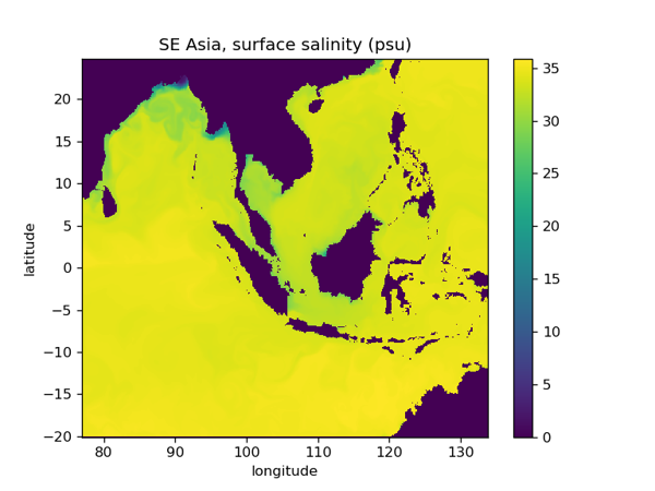
South East Asia, 1/12 deg configuration (ACCORD: SEAsia_R12)
#%%
import coast
import numpy as np
import xarray as xr
import dask
import matplotlib.pyplot as plt
import matplotlib.colors as colors # colormap fiddling

#################################################
#%%  Loading  data
#################################################

dir_nam = "/projectsa/COAsT/NEMO_example_data/SEAsia_R12/"
fil_nam = "SEAsia_R12_5d_20120101_20121231_gridT.nc"
dom_nam = "domain_cfg_ORCA12_adj.nc"
config_t = "/work/jelt/GitHub/COAsT/config/example_nemo_grid_t.json"

sci_t = coast.Gridded(dir_nam + fil_nam, dir_nam + dom_nam, config=config_t)

#%% Plot
fig = plt.figure()

plt.pcolormesh( sci_t.dataset.longitude, sci_t.dataset.latitude, sci_t.dataset.soce.isel(t_dim=0).isel(z_dim=0))
plt.xlabel('longitude')
plt.ylabel('latitude')
plt.title('SE Asia, surface salinity (psu)')
plt.colorbar()
plt.show()
fig.savefig('SEAsia_R12_SSS.png', dpi=120)
Feedback
Was this page helpful?
Glad to hear it!
Sorry to hear that. Please tell us how we can improve.
Last modified December 11, 2023: add configuration gallery (0696a01)